We regroup here all the informations on the Obelisk simulation, as described in the flagship paper.

Initial conditions

The initial conditions for the Obelisk simulation were chosen to follow the high-redshift evolution of an overdense environment. For this purpose, we chose to re-simulate with a high resolution the region around the most massive halo at $z\sim 2$ in the Horizon-AGN simulation: selecting initial conditions based on this simulation allows our results to be compared and contrasted with the work that has already resulted from Horizon-AGN.

The Horizon-AGN simulation follows the evolution of a cosmological volume of side $L_{box} = 100\, h^{-1}$ cMpc (and periodic boundary conditions), assuming a $\Lambda$CDM cosmology compatible with the 7-year data from the Wilkinson Microwave Anistropy Probe (Komatsu et al. 2011): Hubble constant $H_0 = 70.4\,\mbox{km}\,\mbox{s}^{-1}\,\mbox{Mpc}^{-1}$, total matter density $\Omega_{m} = 0.272$, dark energy density $\Omega_{\Lambda} = 0.728$, baryon density $\Omega_{b} = 0.0455$, amplitude of the matter power spectrum $\sigma_8 = 0.81$, and scalar spectral index $n_s = 0.967$. The initial conditions have been created with MPgrafic (Prunet et al. 2008; Prunet & Pichon 2013) with 1024$^3$ DM particles and as many gas cells (corresponding to a DM mass resolution of $M_{DM,HR} = 8 \times 10^7 \, M_\odot$). In the original Horizon-AGN run, the grid is then adaptively refined over the course of the simulation, maintaining a maximum spatial resolution of $\Delta x = 1$ proper kpc at all redshifts down to $z=0$. We improve on this resolution by a factor of ~30 in our Obelisk sub-volume, reaching a resolution of $\Delta$x = 35 pc (more details).

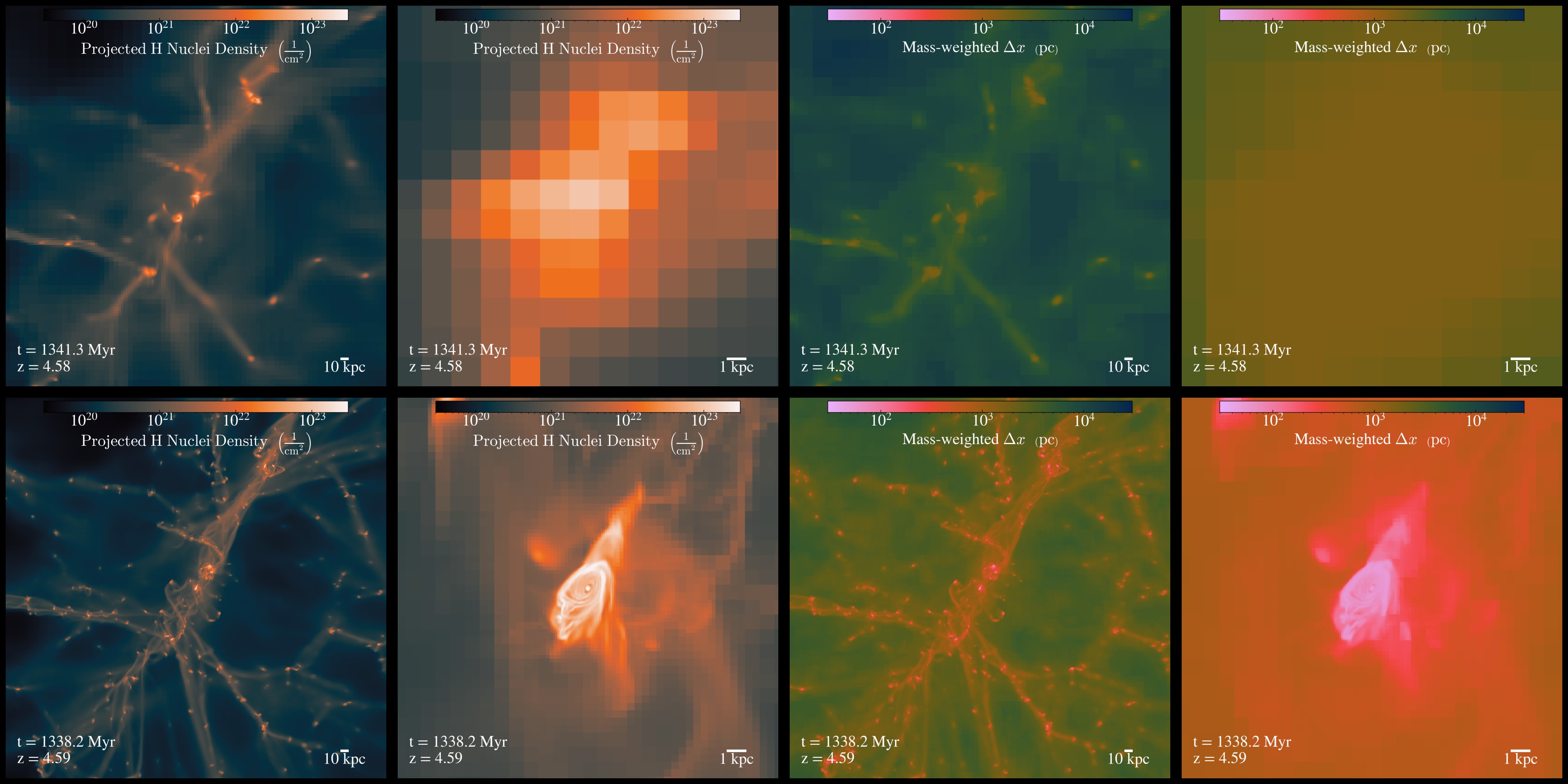
In order to achieve our target resolution at a reasonable computation cost, we only re-simulated a fraction of the initial Horizon-AGN volume. To this end, we selected the most massive halo (of virial mass is around $M_{vir} \simeq 2.5 \times 10^{13}\,M_\odot$) in the simulation at $z \sim 2$ as identified by the [AdaptaHOP]{smallcaps} halo finder (Aubert et al. 2004; Tweed et al. 2009). By $z = 0$, this halo remains the most massive cluster of Horizon-AGN, with $M_{vir} \sim 6.6 \times 10^{14}\,M_\odot$. We first identified all the particles within $4 R_{vir}$ of the target halo at $z = 1.97$, namely in a sphere of radius $2.51\,h^{-1} \mbox{cMpc}$ and tracked them back to the initial conditions. We computed the convex hull enclosing all these particles in the initial conditions and defined this region as our high-resolution patch. We then created a re-sampled version of the Horizon-AGN initial conditions with 4096³ DM particles, corresponding to a mass resolution of $M_{DM,HR} = 1.2\times 10^6\,M_\odot$. Finally, we selected all the high-resolution particles belonging to the patch previously defined, and embedded this patch in the larger Horizon-AGN box, using successively lower and lower resolution regions as buffers, until reaching an effective resolution of 256³ particles in the outer parts of the volume. We filled the full volume with a passive variable whose value is 1 within the high-resolution patch and 0 outside, and used this as a refinement mask (more details). The figure below illustrates the gain in resolution between Horizon-AGN (upper row) and Obelisk (lower row).

Finally, the Obelisk simulation improves upon its parent Horizon-AGN in several important ways (beyond resolution) which we describe in detail further down.

A similar methodology has been employed for the New-Horizon simulation, which focuses on an average region of the Universe. Apart from the radiation-hydrodynamical evolution, our numerical methodology is kept as close as possible to the New-Horizon simulation, so as to facilitate the comparison between the two simulations.

Halo and galaxies

We identified galaxies and haloes in each snapshot of the simulation using the AdaptaHOP halo finder (Aubert et al. 2004; Tweed et al. 2009) with the most massive sub-maximum method (MSM) to separate between host haloes and substructures. In this framework, haloes and subhaloes are groups of particles located at maxima of the density field, and the MSM method requires that the most massive sub-structure is defined as the central object. Compared to previous works using AdaptaHOP (e.g. Dubois et al. 2014a for Horizon-AGN), we amended the halo finder to identify structures using all collisionless particles, both stars and DM. The DM halo is then identified to the DM component of the (sub-)structure, while the galaxy is defined as all stellar particles in the (sub-)structure. In the following, we refer interchangeably to (sub-)structures and (sub-)haloes when discussing groups produced by our modified AdaptaHOP. To be elected as a candidate halo, a structure has to exceed a threshold density $\rho_{t}$. Instead of using a fixed density (e.g. 200 times the average or critical density), we used the fit from Bryan & Norman (1998), yielding an density of roughly $\rho_{t} \lesssim 178$ for the redshift interval studied here. We only considered structures with more than $n_{members} \geq 100$ particles. Notably, we only considered in the analysis galaxies with more than 100 star particles. This yields $52\,428$ ($69\,235$) host haloes, $41\,244$ ($116\,663$) subhaloes and $12\,549$ ($67\,478$) galaxies at $z = 6.0$ ($z = 3.53$), respectively.

Once a (sub-)halo has been identified, we fit a tri-axial ellipsoid to it, and we find the largest ellipsoid for which the virial theorem is verified. We used this ellipsoid to define the virial radius R_vir, and the virial mass M_vir is the mass enclosed in this ellipsoid. In addition to properties global to the total (DM + stellar) structure, we also measured several quantities separately for the stars and DM component, such as the half-mass radius R₅₀. For the galaxy, we also computed additional kinematical and morphological informations such as the projected effective radius R_eff, the star formation rate, or the mass-weighted age and metallicity. We note that a galaxy can correspond to a sub-structure and still lie outside of the virial radius of its parent structure. While we did not separate the populations of central and satellite galaxies in this work, it is worth emphasizing that not all galaxies in sub-structures will correspond to satellite galaxies.

Radiation hydrodynamics

The Obelisk simulation was run with Ramses-RT (Rosdahl et al. 2013; Rosdahl & Teyssier 2015), a multi-group RT extension of the public AMR code Ramses (Teyssier 2002). RAMSES follows the evolution of DM, gas, stars, and BHs, via gravity, hydrodynamics, radiative transfer, and non-equilibrium thermochemistry.

Hydrodynamics and gravity

The gas was evolved using an unsplit second-order MUSCL-Hancock scheme (van Leer 1979), based on the Harten-Lax-van Leer-Contact (HLLC) Riemann solver (Toro et al. 1994) to solve the Euler equations. A MinMod total variation diminishing scheme was used to reconstruct the inter-cell conservative variables from the cell-centred values. We assumed an ideal gas equation of state with adiabatic index $\gamma = 5/3$ to close the relation between internal energy and gas pressure. Gravity was modelled by projecting the collisionless particles (stars and DM) onto the AMR grid using cloud-in-cell interpolation and solving the Poisson equation using the multigrid particle-mesh method described in Guillet & Teyssier (2011) on coarse levels and conjugate gradient on fine levels with a transition at level $\ell = 13$.

In the high-resolution region, the initial mesh was refined up to a spatial resolution of $\Delta x \simeq 35\,\mbox{ckpc}$ (equivalent to 4096³, or an initial grid level $\ell_{min,HR} = 12$), and a passive refinement scalar was set to a value of 1 within that region. We only allowed refinement where the value of this refinement scalar exceeds 0.01, effectively ensuring that only the initial high-resolution region was adaptively refined throughout its collapse. Within this region, we allowed for ten extra levels of refinement, up to a maximal spatial resolution of $\Delta x \simeq 35\,\mbox{pc}$ varying within a factor of two depending on the redshift. Our refinement criterion follows the standard Ramses quasi-Lagrangian approach: A cell is selected for refinement if $\rho_{DM} \Delta x^3 + (\Omega_{DM}/\Omega_b)\rho_{gas} \Delta x^3+ (\Omega_{DM}/\Omega_b) \rho_* \Delta x^3 > 8\ M_{DM,HR}$, where $\rho_{DM}$, $\rho_{gas}$ and $\rho_*$ are the DM, gas and stellar densities in the cell, respectively. In a DM-only run, this would refine a cell as soon as it contains at least eight high-resolution DM particles. We note that cells hosting sink particles and the associated clouds (see the BH section) are always maximally refined. In order to keep the physical resolution constant over the course of the simulation (the box has a constant comoving size), we only permitted a new level of refinement when the expansion scale factor doubles (in our case, a_exp = 0.1 and 0.2). While this is known to induce a small temporary increase in the star formation (e.g. Snaith et al. 2018), it ensures that the physical subgrid models that have been derived with a specific physical resolution in mind are always used at the appropriate scale.

While the baryonic mass (from gas, stars, and BHs) is directly projected onto the maximally refined grid, we smoothed the DM density field by depositing the mass of the DM particles on a coarser grid ($\Delta x \simeq 540\,\mbox{pc}$). This level of smoothing corresponds to the maximal level of refinement triggered in an analogue DM-only simulation where no absolute maximal level of refinement was enforced. This ensures that the effective size of the DM particles correspond to their mass resolution.

The Courant-Friedrichs-Lewy stability condition was enforced using a Courant factor of 0.8, even though the duration of the timestep is predominantly set by the radiation solver (see the next section).

Radiation

The details of the methods used for the injection, propagation, and interaction of the radiation with hydrogen and helium are described in Rosdahl et al. (2013), and we therefore only summarize the main features here.

The RT module propagates the radiation emitted by massive stars and accreting BHs (see the sections on stellar and black-hole radiation for details on the source models) in three frequency intervals describing the HI, HeI, and HeII photon fields (between 13.6 – 24.59 eV, 24.59 – 54.4 eV, and 54.4 – 1000 eV, respectively). The first two moments of the equation of RT are solved on the AMR grid using an explicit first-order Godunov method with the M1 closure (Dubroca & Feugeas 1999; Levermore 1984) for the Eddington tensor. The radiation is then coupled to the hydrodynamical evolution of the gas through the non-equilibrium thermochemistry for hydrogen and helium and radiation pressure (more details).

As we used an explicit solver, we are subject to a Courant-like condition for the propagation of the radiation. This is an extremely stringent condition for the radiation: as the speed of light is much larger than any other velocity in the simulation, the RT timestep should in principle be extremely short. We mitigated this in two ways, following a similar approach to the Sphinx simulation (Rosdahl et al. 2018). First, subcycled the RT timestep on each AMR level, with up to 500 RT steps for each hydro step, while preventing photons from crossing level boundaries during the subcycling (see the discussion in section 2.4 of Rosdahl et al. (2018)). In addition to this, we used the traditional approach of artificially reducing the speed of light by a constant factor, $f_c$, to prevent too short a timestep and too large a number of RT subcycles. This “reduced speed of light” approximation, initially proposed by Gnedin & Abel (2001) and used here following the implementation of Rosdahl et al. (2013), works well when studying the ISM and the CGM of individual galaxies, where the propagation of light is effectively limited by the propagation of ionization fronts. Contrary to single galaxy or small volume simulations performed with Ramses-RT (Costa et al. 2019; e.g. Kimm et al. 2017; Trebitsch et al. 2017), the Obelisk simulation tracks the reionization process in a reasonably large volume of the Universe (typically $\gtrsim 10^4\,\mbox{Mpc}^3$ comoving at $z \sim 4$): Because of this we can no longer fully employ this reduced speed of light approximation. We instead used the so-called ‘variable speed of light’ approximation (VSLA, Katz et al. 2017), where the factor $f_c$ is local. Ideally, one would have a relatively low speed of light in the densest regions and a higher speed of light in voids. With our quasi-Lagrangian refinement strategy, this can be achieved by tying the reduction factor to the cell size; with a cell twice as small as its neighbour will use a value of $f_c$ reduced by a factor of two. Following Katz et al. (2018) and the simulation, we used $f_c = 0.2$ for the coarsest cells in the high-resolution region ($\ell = 12$ or $\Delta x \simeq 35\,\mbox{ckpc}$) as the reionization history should be fairly converged with this value (e.g. Deparis et al. 2019; Ocvirk et al. 2019). We then chose to decrease $f_c$ by a factor of two per level until $f_c = 0.0125$ at all levels above $\ell \geq 16$ ($\Delta x \simeq 2\,\mbox{kpc}$). For the low resolution cells outside of the high-resolution region, we set the speed of light to a low value ($f_c = 0.01$). While this creates some accumulation of radiation just outside of the region of interest, the effects on the high-resolution region are negligible.

As one of the major endeavours of the Obelisk project is to study the relative contributions of massive stars and of AGN to the establishment and maintenance of the ionizing UV background, we used the photon tracer algorithm of (Katz et al. 2018; Katz et al. 2019a) to keep track of the contribution of different sources to the local photon flux (and hence the strength of the UV background) and ionization of the gas. In a nutshell, we track the fractional contribution of each type of source to the radiation density and flux when the photons are injected and advected on the grid. With this, we also keep track of the fraction of the gas that has been photoionized by each type of source, and the difference with the total HII fraction in each cell is the fraction of the gas that has been collisionally ionized. This allows us, for example, to track across cosmic time which sources contribute the most to HI-photoionization rate in the IGM, which sources are responsible for ionizing which environment, and to compute population-averaged escape fractions. This algorithm has already been applied in Katz et al. (2018) and Katz et al. (2019b) to study the contribution to reionization of stellar sources of different ages or mass, or residing in haloes of difference masses. In this work, we traced photons based on their original source: We explicitly follow the radiation produced by stellar populations and by accreting BHs. More details can be found in the Sect. 2 of Katz et al. (2018) for details on the implementation of the algorithm.

Thermochemistry

Ramses-RT features non-equilibrium thermochemistry by following the ionization state of hydrogen and helium: H, H⁺, He, He⁺, He⁺⁺, as described in Rosdahl et al. (2013). The coupling with the radiation is performed via photoionization, collisional ionization, collisional excitation, recombination, bremsstrahlung, homogeneous cooling and heating off the cosmic microwave background, and di-electronic recombinations. The whole thermochemistry step is subcycled within every RT step, and uses the smooth injection approach from Rosdahl et al. (2013) to limit the amount of subcycling. We further assume the on-the-spot approximation: Any ionizing photon emitted by recombination is assumed to be absorbed locally, and we thus ignore emission of ionizing radiation resulting from direct recombinations to the ground level.

We include a cooling contribution from metals using the standard approach in Ramses. Above $T \geq 10^4\,\mbox{K}$, we use the cooling rates computed with Cloudy (version 6.02, Ferland et al. 1998) assuming photoionization equilibrium with the redshift-dependent Haardt & Madau (1996) UV background. We stress that we do not use this UV background for the hydrogen and helium non-equilibrium photo-chemistry, but solely for computing the metal cooling rates. We also account for energy losses via metal line cooling below $T \leq 10^4\,\mbox{K}$, following the prescription of Rosen & Bregman (1995) based on Dalgarno & McCray (1972), and approximate the effect of the metallicity by scaling the metal cooling enhancement linearly (we still assume a Solar-like abundance pattern for simplicity). This allows the gas to cool down to a temperature floor of $T_{floor} = 50\,\mbox{K}$. We chose to use a density-independent temperature floor rather than a (density-dependent) pressure floor, usually used to prevent numerical fragmentation (Truelove et al. 1998), because our model for star formation (see the next section) is constructed to efficiently remove gas to form stars in regions with high density and low temperature (which would be susceptible to numerical fragmentation).

Because we do not include molecular hydrogen, we adopted a homogeneous initial metallicity floor of $Z = 10^{-3} Z_\odot$ in the whole computational volume, to allow the gas to cool down below $10^4\,\mbox{K}$ before the formation of the first stars (and the subsequent metal enrichment). Aside from this, the gas in the box is initially neutral and composed of $X=76\,\%$ hydrogen and $X=24\,\%$ helium by mass.

Stellar populations

We model stars as particles with mass $m_\star \simeq 10^4\,M_\odot$ representing a single stellar population, assuming a fully sampled Kroupa (2001) initial mass function (IMF) between $0.1$ and $100\,M_\odot$.

Star formation

We only consider cells to be star forming when the local number density $n_{gas}$ (or equivalently the mass density $\rho_{gas}$) exceeds a threshold $n_{SF} = 5\,\mbox{H}\,\mbox{cm}^{-3}$ (chosen as the typical ISM density), and when the local turbulent Mach number defined as the ratio of the turbulent velocity to the sound speed exceeds $\mathcal{M} \geq 2$. The amount of gas converted into stars follows a Schmidt (1959) law:

$$\dot{\rho}_{\star} = \varepsilon_{\star} \frac{\rho_{gas}}{t_{ff}},$$

so that on average $M_{sf} = \dot{\rho}_\star \Delta x^3 \Delta t = \varepsilon_{\star} \rho_{gas} \Delta x^3 \Delta t/t_{ff}$ of gas is converted into star particles during one timestep $\Delta t$, where $G$ is the gravitational constant, $\varepsilon_{\star}$ is the local star formation efficiency per free-fall time and $t_{ff} = (3\pi / 32 G \rho_{gas})^{1/2}$ is the gas free-fall time.

One key difference between the method we use here, as already discussed for example in Trebitsch et al. (2017) or Kimm et al. (2017), and the traditional approach used for instance in Horizon-AGN is that the star formation efficiency $\varepsilon_{\star}$ is a local parameter, rather than a constant, and depends on the local gas density $\rho_{gas}$, sound speed $c_{s}$, and turbulent velocity $\sigma_{gas}$. Here, we approximated $\sigma_{gas}$ by taking the velocity differences between the host cell and its immediate neighbours. The analytic expression for $\varepsilon_{\star}(\rho_{gas}, c_s, \sigma_{gas})$ follows the ‘multi-ff PN’ model of Federrath & Klessen (2012) and Padoan & Nordlund (2011):

$$\varepsilon_{\star} \propto \text{e}^{\frac{3}{8}\sigma_s^2}\left[1 + \mbox{erf}\left(\frac{\sigma_s^2 - s_{\mbox{crit}}}{\sqrt{2\sigma_s^2}}\right)\right],$$

for $\mathcal{M} \geq 2$ and $0$ otherwise, and where $\sigma_s = \sigma_s(\sigma_{gas}, c_{s})$ characterizes the turbulent density fluctuations, $s_{crit} = \mbox{ln}(\rho_{gas, crit}/\rho_{gas})$ is the critical density above which the gas will be accreted onto stars, and $\rho_{gas, crit} \propto (\sigma_{gas}^2 + c_{s}^2) \sigma_{gas}^2/c_{s}^2$. In practice, this means that $\varepsilon_\star$ increases with $\sigma_{gas}$, and when the virial parameter decreases.

The actual number $N$ of particles formed in one cell in one timestep $\Delta t$ is drawn from a Poisson distribution $P(N) = (\lambda^N/N!) e^{-\lambda}$ of parameter $\lambda = M_{sf} / m_\star$ (see Rasera & Teyssier 2006 for details). Additionally, for numerical stability, we limit the number of star particles formed in one timestep so that the amount of gas removed from a cell is capped at $90\%$ of the gas mass in that cell.

Supernova feedback

When a star particle reaches an age of $t_{\mbox{SN}} = 5\,\mbox{Myr}$, we assume that a mass fraction $\eta_\mbox{SN} = 0.2$ of the initial stellar population explodes as SNe and returns mass and metals to its environment with a yield of $0.075$. Each SN explosion releases an energy $E_\mbox{SN} = 10^{51}\,\mbox{erg}$ assuming an average progenitor mass of $m_\mbox{SN} \simeq 20\,M_\odot$, corresponding to an average of 1 SN explosion for $100\,M_\odot$ of stars. At our mass resolution, each star particle releases $10^{53}\,\mbox{erg}$ per event, instantaneously.

The explosion itself was modelled following the mechanical feedback implementation of Kimm & Cen (2014), Kimm et al. (2015), which injects radial momentum according to the phase of the explosion (energy conserving or momentum conserving) that is resolved. We refer the reader to these works for the details of the algorithm implementation, and once again only recall the main features here. If we resolve the adiabatic expansion phase of the SN, we directly inject the kinetic energy and momentum corresponding to $10^{51}\,\mbox{erg}$ to the cells neighbouring the SN site. If this energy conserving phase is not resolved, the SN explosion is only captured in its final snowplough phase; in this case we directly inject the terminal momentum $p_\mbox{snow}$ in the neighbouring cells. We determine the phase of the SN explosion that we resolved on a cell-by-cell basis: For each of the cells neighbouring the SN site, we evaluate the mass ratio $\chi_\mbox{SN} = \mbox{d}M_\mbox{swept} / \mbox{d}M_\mbox{ej}$ between the swept material (ejecta + swept ISM) and the ejecta, and compare it to a critical mass ratio $\chi_{\mbox{SN,tr}}$. For low values of $\chi_\mbox{SN}$ (i.e. in the adiabatic phase), we inject

$$\Delta p_\mbox{ad} = f_\mbox{geom} \sqrt{2\chi_\mbox{SN} M_\mbox{ej} f_\mbox{e} E_\mbox{SN}},$$

where $f_\mbox{geom}$ is a geometrical factor describing how the total energy and mass of the SN is split between the neighbouring cells, and $f_\mbox{e} = 1 - (\chi_\mbox{SN} -1)/(3\chi_{\mbox{SN,tr}} -1)$ ensures a smooth transition between the two modes of momentum injection. In the snowplough phase, we inject the terminal momentum (Blondin et al. 1998; Kim & Ostriker 2015; Martizzi et al. 2015; e.g. Thornton et al. 1998)

$$\Delta p_\mbox{snow} = 3\times 10^{5}\,M_\odot\,\mbox{km}\,\mbox{s}^{-1}\, f_\mbox{geom} E_{\mbox{SN},51}^{16/17} n_{H}^{-2/17} \tilde{Z}^{-0.14},$$(1)

where $E_{\mbox{SN},51}$ is the total SN energy in units of $10^{51} \,\mbox{erg}$, $n_{H}$ is the local hydrogen number density in units of $\mbox{cm}^{-3}$, and $\tilde{Z}$ is the local metallicity in units of $Z_\odot$ floored at $0.01\, Z_\odot$.

We further assumed that, the photo-ionization pre-processing of the ISM by young OB stars prior to the SN event augments the final radial momentum from a SN (Geen et al. 2015). While this should be taken into account by the radiative transfer in our simulation, Trebitsch et al. (2017) argued that a significant fraction of the ionizing radiation can be emitted in regions where the Strömgren radius, $r_S$, is not resolved in which case this momentum increase will often be missed. Thus, as in Trebitsch et al. (2018) and Rosdahl et al. (2018), we followed the subgrid model of Kimm et al. (2017), which adds this missing momentum when the Strömgren radius is locally not resolved, when $r_S < \Delta x$. We then increased the pre-factor in eq. 1 to $5 \times 10^{5}\,M_\odot\,\mbox{km}\,\mbox{s}^{-1}$ following the results of Geen et al. (2015).

Stellar radiation

Using the Sphinx simulation, Rosdahl et al. (2018) have shown that the inclusion of binary stars has a strong effect on the timing of reionization because binary interactions lead to an increased and more sustained production of ionizing radiation (Götberg et al. 2019; e.g. Stanway et al. 2016; but see also Topping & Shull 2015). We emit ionizing radiation from each star particle following the spectral energy distribution (SED) resulting from the Binary Population and Spectral Synthesis code v2.2.1 (Bpass, Eldridge et al. 2017; Stanway & Eldridge 2018, Tuatara version), which includes the effect of these binary interactions. In the Tuatara release, the binary fraction of stars depends on the initial stellar mass, with around 60% (6%) of low-mass (high-mass) stars being isolated. More specifically, we used the model imf135_100 closest to a Kroupa (2001) IMF with slopes $-1.30$ between $0.1 - 0.5\,M_\odot$ and $-2.35$ between $0.5 - 100\,M_\odot$. Each star particle is assigned a luminosity in each radiation bin as a function of its age and metallicity, scaled directly with the mass of the particle. As described in Rosdahl et al. (2013), the average energy of each radiation bin and the interaction cross-sections are updated every five coarse timesteps, so that they accurately represent the properties of the average source population.

While lower resolution simulations usually include a subgrid correction to account for the unresolved escape fraction and calibrated to reproduce reasonable reionization history (Finlator et al. 2018; e.g. Gnedin et al. 2014; Ocvirk et al. 2016, 2020; Pawlik et al. 2017), we followed here the approach taken by simulations reaching a spatial resolution better than a few tens of parsecs and use the luminosity of the star particle directly. We stress that we do not claim that $\Delta x \simeq 35\,\mbox{pc}$ is sufficient to resolve in great detail the rich multi-phase structure of the ISM; we acknowledge that the uncertainty on the ISM structure could affect the escape of ionizing radiation from birth clouds either way: Unresolved ionized channels could lead to a higher escape fraction (e.g. Ma et al. 2015), while unresolved clumping could increase the amount of absorption in the ISM (e.g. Yoo et al. 2020). We note however that the tests performed in the Sphinx framework (appendix B of Rosdahl et al. 2018) suggest that a resolution of $\Delta x \simeq 20\,\mbox{pc}$ yields galaxy properties similar to their fiducial run with $\Delta x \simeq 10\,\mbox{pc}$.

Finally, we note that the absence of subgrid calibration of the escape fraction is consistent with the assumptions we made for the star formation model and for the BH accretion (see the next section): namely, that we broadly resolve the large-scale ISM density distribution and the formation of molecular clouds. Changing one ingredient (e.g. the unresolved escape of radiation) without changing the others would break that consistency.

Black holes

We followed the same approach to model BHs, based on the implementation of Dubois et al. (2010), Dubois et al. (2012) Dubois et al. (2014c): BHs are modelled as sink particles, which are allowed to accrete gas and release energy, momentum and radiation into their environment. We shall now describe the various aspects of our BH model.

BH formation

We seeded the sink particles representing our BHs with an initial mass $M_{\bullet,0} = 3 \times 10^4\,M_\odot$ in cells where the following criteria are met: the gas density $n_{\mbox{gas}}$ and stellar density $n_\star$ must both locally exceed a threshold $n_{\mbox{sink}} = 100\,\mbox{H}\,\mbox{cm}^{-3}$; and the gas must be Jeans-unstable. We imposed an exclusion radius $r_{\mbox{excl}} = 50\,\mbox{kpc}$ to avoid the formation of multiple BHs in the same galaxy. Each sink particle is dressed with a swarm of `cloud’ particles, positioned on a regular grid lattice within a sphere of radius $4 \Delta x$ and equally spaced by $\Delta x/2$. These cloud particles provide a convenient way of probing and averaging the properties of the gas around the BH. At our resolution, this means we probe a sphere of radius $4\Delta x \simeq 140\,\mbox{pc}$ around each BH with 2109 clouds. We set the initial velocity of the BH to that of its host cell, and assigned it a spin $a = 0$.

Our seed mass choice stems from physical as well as numerical considerations. The BH formation mechanism is highly uncertain, with different models predicting very different seed masses, from $\sim 10\,M_\odot$ to $\gtrsim 10^5\,M_\odot$ (e.g. Volonteri 2010). Numerically, having a BH seed less massive than the mass of star particles is not desirable: Pfister et al. (2019) suggests that otherwise, the BH trajectory becomes extremely sensitive to the fluctuation of the (stellar) gravitational potential. As our mass resolution for star particles is $m_\star \simeq 10^4\,M_\odot$, we choose a BH seed mass three times higher. The underlying physical picture would be that of a light seed BH that has already undergone some early growth or of a heavier seed, and is consistent with our choice of seeding BHs only in regions with a sufficiently high stellar density (thus mimicking pre-galactic centres).

BH accretion

Once a sink particle has formed, it grows through two channels: BH-BH mergers and gas accretion. We allowed two BHs to merge when they are closer than $4\Delta x$ from one another, and only if their relative velocity is lower than the escape velocity of the binary system they would form in vacuum. As we are far from resolving the gaseous accretion disc around BHs, we used the classical Bondi-Hoyle-Lyttleton (Bondi 1952) approach to compute the accretion rate onto the BH:

$$\dot{M}_{\mbox{BHL}} = 4\pi G^2 M_{\bullet}^2 \frac{\bar{\rho}}{\left(\bar{c}_s^2 + \bar{v}_{\mbox{rel}}^2\right)^{3/2}}\,,$$(2)

where $M_{\bullet}$ is the BH mass, $\bar{\rho}$ and $\bar{c}_s$ are respectively the average gas density and sound speed, and $\bar{v}_{\mbox{rel}}$ is the relative velocity between the BH and the surrounding gas. The bar notation denotes an averaging over the cloud particles using a Gaussian kernel $w \propto \exp\left(-r^2/r_{\mbox{sink}}^2\right)$, where $r_{\mbox{sink}}$ is defined using the Bondi radius $r_{\mbox{BHL}} = \frac{GM_{\bullet}}{c_s^2 + v_{\mbox{rel}}^2}$:

$$\label{eq:rsink} r_{\mbox{sink}} = \begin{cases} \Delta x/4 & \text{if}\quad r_{\mbox{BHL}} < \Delta x/4, \\ r_{\mbox{BHL}} & \text{if}\quad \Delta x/4 \leq r_{\mbox{BHL}} < 2 \Delta x, \\ 2 \Delta x & \text{if}\quad 2 \Delta x \leq r_{\mbox{BHL}}. \end{cases}$$

We did not use any extra artificial boost for the gas accretion onto the BH. The accretion rate was capped at the Eddington rate:

$$\dot{M}_{\mbox{Edd}} = \frac{4\pi G M_{\bullet} m_p}{\varepsilon_r \sigma_{\mbox{T}} c}, \label{eq:accrate-edd}$$

where $m_p$ is the proton mass, $\sigma_{\mbox{T}}$ is the Thompson cross section, $c$ is the speed of light and $\varepsilon_r$ is the radiative efficiency of the accretion flow onto the BH, which depends on the spin of the BH (see the section on BH spin). Additionally, only a fraction $1-\varepsilon_r$ of the mass accreted onto the accretion disc effectively reaches the BH: The rest is radiated away. At very low accretion rates, when $\chi = \dot{M}_{\mbox{BHL}}/\dot{M}_{\mbox{Edd}}$ drops below $\chi_{\mbox{crit}} = 0.01$, the flow becomes radiatively inefficient, in which case we followed eq. 16 of Benson & Babul (2009) and reduce the radiative efficiency of the flow to $\tilde{\varepsilon_{r}} = \varepsilon_r (\chi/\chi_{\mbox{crit}})$. The final BH accretion rate is therefore:

$$\label{eq:accrate-both} \dot{M_{\bullet}} = (1-\tilde{\varepsilon_r}) \min\left(\dot{M}_{\mbox{BHL}}, \dot{M}_{\mbox{Edd}}\right).$$

Gas is then removed from cells within $4 \Delta x$ of the sink particle in a kernel-weighted fashion, and the accretion is capped to prevent the BH from removing more than 25% of the gas content of the cell in one timestep for numerical stability (i.e. $w \dot{M_{\bullet}}\Delta t \lesssim 0.25 \rho_{\mbox{gas}}\Delta x^3$).

BH dynamics

While the dynamics of the sink particles is computed at the most refined grid level (see here), we lack the resolution to accurately capture the effects of dynamical friction that will affect the detailed BH dynamics. For instance, Pfister et al. (2017) showed with a resolution study that resolving the influence radius of a BH is crucial to get a chance to resolve the formation of BH binaries in the aftermath of a galaxy merger; this length-scale being of the order of $1\,\mbox{pc}$ for a BH with mass $M_{\bullet} \sim 10^6\,M_\odot$ in a Milky-Way-like galaxy, and much lower for less massive BHs, it is well below the resolution that modern cosmological simulations such as Obelisk can reach. While most of these simulations resort to moving the sink particle towards a local minimum of the potential (e.g. Crain et al. 2015; Davé et al. 2019; Pillepich et al. 2018), we took here a different approach and used a subgrid model to account for the effect of the unresolved dynamical friction (see also Tremmel et al. 2015).

We used the drag force implementation introduced in Dubois et al. (2013) to model the force exerted by the gaseous wake lagging behind the BH. The frictional force has an analytic expression given by Ostriker (1999), and is proportional to $F_{\mbox{DF}} = \alpha f_{\mbox{gas}} 4\pi \rho (G M_{\bullet} / \bar{c_s}^2)$, where $\alpha$ is an artificial boost, with $\alpha = (\rho/\rho_{\mbox{DF, th}})^2$ if $\rho > \rho_{\mbox{th}}$ and 1 otherwise, and $f_{\mbox{gas}}$ is a fudge factor varying between 0 and 2 which depends on the BH Mach number $\mathcal{M}_\bullet = \bar{v}_{\mbox{rel}}/\bar{c}_s$ (Chapon et al. 2013; Ostriker 1999). In light of the results of Beckmann et al. (2018) who showed that this subgrid model begins to fail when the wake is resolved, we set $F_{\mbox{DF}} = 0$ whenever the influence radius $2\mbox{G} M_\bullet / \max(\bar{c_s},\bar{v_\mbox{rel}})^2 > 0.2\Delta x$. In this work, we took $\rho_{\mbox{DF, th}} \simeq 0.003\ \mbox{to}\ 0.01 \,\mbox{cm}^{-3}$. We discuss the effect of this ad hoc choice in an appendix of the paper.

We also included a contribution to the dynamical friction caused by collisionless particles (stars and DM separately), analogous to what happens to the gas: A gravitational wake of stars and DM is created by the passage of a massive body (the BH) and will decelerate it (Binney & Tremaine 1987; Chandrasekhar 1943). Our implementation, described in detail in Pfister et al. (2019), is somewhat similar to that of Tremmel et al. (2015) used in the simulation (Tremmel et al. 2017). We directly compute the contribution of the collisionless particles within a sphere of radius $4\Delta x$. The deceleration is parallel to the velocity $\mathbf{v}_\bullet$ of the BH relative to the background (stars and DM) and has a magnitude $a_{\mbox{DF}}$ is computed as follow:

$$\label{eq:aDF-chandra} a_{\mbox{DF}} = -4\pi \frac{G^2 M_{\bullet}}{v_\bullet^2} \left( \log\Lambda \int_0^{v_\bullet} 4\pi v_\bullet^2 f(v) \mbox{d}v + \int_{v_\bullet}^\infty 4\pi v^2 f(v) \left[\log\left(\frac{v+v_\bullet}{v-v_\bullet}\right) - 2\frac{v_\bullet}{v}\right] \mbox{d}v \right)\,,$$

where $v_\bullet$ is the norm of the relative velocity with respect to the mass-weighted velocity of the surrounding collisionless particles, $\Lambda = 4\Delta x / r_{\mbox{def}}$ is the Coulomb logarithm with $r_{\mbox{def}} = GM_{\bullet}/v_\bullet^2$, and $f$ is the distribution function defined with the velocities of the particles withing the sphere of radius $4\Delta x$. As for the gas, we switch off the subgrid model when the influence radius is resolved by more than $0.2\Delta x$

$$\label{eq:distribfunction} 4\pi v^2 f(v) = \frac{3}{256\pi \Delta x^3}\sum_i m_i \delta(v_i - v).$$

We refer the interested reader to Pfister et al. (2019) for a more detailed discussion of the model.

BH spin evolution

We follow self-consistently the evolution of the spin magnitude and direction over the course of the simulation using the implementation presented in Dubois et al. (2014b) and Dubois et al. (2014c) (but see also Fiacconi et al. (2018); Bustamante & Springel (2019) for similar implementations). Here again, we refer the interested reader to these works for an extensive discussion of the model and tests of its validity.

We evolve the magnitude of the spin following gas accretion through an expression derived in Bardeen (1970):

$$\label{eq:spinevol-bardeen} a^{n+1} = \frac{1}{3} \frac{r_{\mbox{isco}}^{1/2}}{M_{\mbox{ratio}}} \left[4 - \left(3\frac{r_{\mbox{isco}}}{M_{\mbox{ratio}}^2} - 2\right)^{1/2}\right],$$

where $M_{\mbox{ratio}} = M_{\bullet}_{,n+1}/M_{\bullet}_{,n}$ ($M_{\bullet}_{,n}$ being the mass of the BH at times $t_n$), and

$$r_{\mbox{isco}} = R_{\mbox{isco}}/R_{\mbox{g}} = 3 + Z_2 \mp \operatorname{sign}(a) \sqrt{(3-Z_1)(3+Z_1+2Z_2)}$$(3)

is the radius of the innermost stable circular orbit (ISCO) expressed in units of gravitational radius $R_{\mbox{g}}$. $Z_1$ and $Z_2$ are function of the spin magnitude $a$, given by

$$\label{eq:spinZ1} \begin{aligned} Z_1 &= 1 + (1-a^2)^{1/3}\left[(1+a)^{1/3} + (1-a)^{1/3}\right] \\ Z_2 &= \left(3a^2 + Z_1^2\right)^{1/2}. \end{aligned}$$

The $\mp$ sign in eq. 3 depends on whether the BH is co-rotating ($a \geq 0$) or counter-rotating ($a \leq 0$) with its accretion disc. For a co-rotating BH, $1 \leq r_{\mbox{isco}} \leq 6$, while $6 \leq r_{\mbox{isco}} \leq 9$ for the counter-rotation case ($r_{\mbox{isco}} = 6$ only for a non-spinning BH). The direction of the BH spin is evolved assuming that the angular momentum of the (unresolved) accretion disc aligns with that of the accreted gas. The potential mis-alignment between the BH spin and the accretion disc leads to the formation of a warped disc in the innermost regions of the accretion disc precessing about the spin axis because of the Lense-Thirring effect. This warped disc will eventually completely align or anti-align with the BH spin. The anti-alignment configuration occurs when the angle $\theta$ between angular momenta of the disc $\mathbf{J_{\mbox{d}}}$ and of the BH $\mathbf{J_{\bullet}}$ fulfils $\cos\theta < -0.5 \|\mathbf{J_{\mbox{d}}}\| / \|\mathbf{J_{\bullet}}\|$ (King et al. 2005). We assume that the accretion disc is well described by the Shakura & Sunyaev (1973) thin disc, and define $J_{\mbox{d}}$ as the value of the angular at the smallest radius between the warp radius and the self-gravity radius. We refer the reader to Sect. 3 of Dubois et al. (2014c) for the equations governing the details of this process, but we wish to stress here that we do not enforce the spin of the BH to always be aligned with the angular momentum of the accreted gas.

Our model assumes a thin disc solution: We only apply it at high accretion rates, when $\chi \gtrsim 0.01$. At lower accretion rate, when the accretion flow is radiatively inefficient, we modify our model following the results of the simulations of ‘magnetically choked’ accretion flows from McKinney et al. (2012). In practice, we assume that each low accretion rate event fills an accretion disc, and over the course of the accretion event, the BH spin is evolved at a rate given by a `spin-up’ parameter (or rather spin-down parameter, as in this regime, the absolute value of the spin magnitude tends to decrease systematically) given by a fourth-order polynomial fit of the results in Table 7 of McKinney et al. (2012), particularly their simulations where is the BH spin of each model. In any case, we limit the spin-up process to $|a| \leq a_{\mbox{max}} = 0.998$ following Thorne (1974). Finally, when two BHs merge, we update the spin of the remnant using the fit of Rezzolla et al. (2008), according the measured pre-merger BH spins, orbital angular momentum, and mass ratio.

The spin evolution is not a purely passive quantity in Obelisk: The radiative efficiency $\varepsilon_r$ of the accretion flow is effectively set by the spin through $r_{\mbox{isco}}$:

$$\label{eq:effrad} \varepsilon_r = 1 - \sqrt{1 - \frac{2}{3r_{\mbox{isco}}}}.$$

For a non-rotating BH, this leads to $\varepsilon_r \simeq 0.057$, and the canonical $\varepsilon_r = 0.1$ corresponds to $a \simeq 0.7$.

AGN feedback

We implemented AGN feedback following accretion events using the dual mode approach of Dubois et al. (2012). At low Eddington ratio $\chi < \chi_{\mbox{crit}}$, the AGN is in ‘radio mode’, while it is in ‘quasar mode’ when $\lambda_{\mbox{Edd}} \geq 0.01$.

For the quasar mode, each sink particle dumps an amount $\dot{E}_{\mbox{AGN}} \Delta t$ of thermal energy over a timestep $\Delta t$ in a sphere of radius $\Delta x$ centred on the BH. The energy injection rate is calculated as

$$\label{eq:Edot_quasar} \dot{E}_{\mbox{AGN}} = \varepsilon_f \varepsilon_r \dot{M}_\bullet c^2,$$

where $\varepsilon_f = 0.15$ is the fraction of the bolometric luminosity that is transferred to the gas (Booth & Schaye 2009; Dubois et al. 2012) , driving unresolved winds through Compton heating, and UV and IR momentum coupling of radiation. This ad hoc choice efficiency allows for the self-regulation of BH growth through their feedback. The actual input of (UV) photons from the AGN is also treated explicitly on resolved scales with the Ramses-RT solver (see the next section).

For the radio mode, we deposit momentum as a bipolar cylindrical outflow mimicking the propagation of a jet in the surrounding gas with a velocity $u_{\mbox{J}} = 10^4\,\mbox{km}\,\mbox{s}^{-1}$. The outflow profile corresponds to a cylinder of radius $\Delta x$ and height $2\Delta x$ weighted by a kernel function

$$\label{eq:jetprofile} \psi\left(r_{\mbox{cyl}}\right) = \frac{1}{2\pi\Delta x^2}\exp\left(-\frac{r_{\mbox{cyl}}^2}{\Delta x^2}\right),$$

with $r_{\mbox{cyl}}$ the cylindrical radius. The outflow removes mass from the central cell and transport it to the cells enclosed by the jet at a rate $\dot{M}_{\mbox{J}}$ with

$$\label{eq:jetmass} \dot{M}_{\mbox{J}}(r_{\mbox{cyl}}) = \frac{\psi(r_{\mbox{cyl}})}{\Psi} \eta_{\mbox{J}} \dot{M}_\bullet\,,$$

where $\Psi$ is the integral of $\psi$ over the cylinder and $\eta_{\mbox{J}} = 100$ is the mass-loading factor of the jet accounting for the interaction between the jet and the ISM at unresolved scales. The momentum is injected in a direction parallel to the BH spin (with opposite signs above and below the sink) with the norm of the momentum $q(r_{\mbox{cyl}})$ given by

$$\label{eq:jetmomentum} q_{\mbox{J}}(r_{\mbox{cyl}}) = \dot{M}_{\mbox{J}}(r_{\mbox{cyl}}) u_{\mbox{J}}.$$

We inject the corresponding kinetic energy into the gas:

$$\label{eq:jetegy} \dot{E}_{\mbox{J}}(r_{\mbox{cyl}}) = \frac{q_{\mbox{J}}(r_{\mbox{cyl}})^2}{2 \dot{M}_{\mbox{J}}(r_{\mbox{cyl}})} = \frac{\psi(r_{\mbox{cyl}})}{\Psi} \dot{E}_{\mbox{AGN}}.$$

Here, the injection rate $\dot{E}_{\mbox{AGN}}$ is given by

$$\label{eq:Edot_radio} \dot{E}_{\mbox{AGN}} = \varepsilon_{\mbox{MCAF}} \dot{M}_\bullet c^2,$$

where $\varepsilon_{\mbox{MCAF}}$ is given by a fourth-order polynomial fit to the simulations of McKinney et al. (2012). More precisely, we use the same set of simulations as for the spin evolution (see the section on BH spin), and sum the contributions of winds and jet based on Table 5: $\varepsilon_{\mbox{MCAF}} = \varepsilon_{\mbox{j}} + \varepsilon_{\mbox{w,o}}$ (using respectively $\eta_{\mbox{j}}$ and $\eta_{\mbox{w,o}}$ in their notations).

BH radiation

In addition to the thermal and kinetic energy injection described in the previous section, we release ionizing energy radiation from the BHs to represent the contribution of AGN to the ionizing radiation field. For this, we applied the method presented in Trebitsch et al. (2019). We release radiation at each fine timestep, and the amount of radiation released in each frequency bin is given by the luminosity of the quasar in each band. In this section, we highlight the main aspects of our AGN SED model. [TODO: add appendix here]

Overview

While the implementation of the photon injection is similar to the work of Bieri et al. (2017), it differs in the spectrum assumed for the AGN. Indeed, instead of a constant SED inspired by the averaged spectrum of Sazonov et al. (2004), we modelled the SED of the radiation produced by the accretion onto the BH as a multi-colour black-body spectrum corresponding to a Shakura & Sunyaev (1973) thin disc, and extend it at high energy with a power-law $\alpha_{\mbox{UV}} = -1.5$, consistent with the value derived by Lusso et al. (2015) for a sample of high-redshift quasars. We then approximated the whole spectrum with a piecewise power-law for simplicity. We assume that $f_{\mbox{IR}} = 30\%$ (consistent with the Sazonov et al. (2004) spectrum) of the bolometric luminosity of the disc is absorbed by dust and re-emitted as IR radiation (which will participate to the quasar mode feedback), which we do not model here, thus leaving a total luminosity $L_{\mbox{rad}} = 0.7 \varepsilon_r \dot{M_{\bullet}} c^2$ available for the radiation. To get the AGN luminosity in each frequency bin, we integrate the resulting SED in each frequency interval. Similarly, we compute the average photon energy in each bin, as well as the energy-weighted and photon-weighted interaction cross sections (see Rosdahl et al. (2013) for details on the role of these quantities). We do not include the presence of X-rays, which can create a diffuse shell of partially ionized gas in the outskirts of cosmological regions (Graziani et al. 2018).

As the disc profile is a function of $M_{\bullet}$, $\dot{M_{\bullet}}$ and $a$, the multi-colour black-body spectrum of the AGN will also depend on these parameters. To limit the computational cost, we pre-calculate all the quantities that depend on the AGN SED, and only interpolate between these values over the course of the simulation. Because the shape of the spectrum is weakly sensitive to the value of the spin parameter, we adopt the shape corresponding to $a = 0$. We have ensured that the adopted AGN SED yields an average spectrum similar to the AGN SED used in Volonteri et al. (2017) for a population of growing BHs at $z \sim 6$.

Finally, we note again that the thin disc solution assumes that the accretion flow is radiatively efficient: We therefore only release radiation when $\chi \geq \chi_{\mbox{crit}}$.

AGN SED

We highlight that our endeavour here is not to provide an AGN spectrum comparable with observations on a one-to-one basis, but rather to derive a spectral shape that will broadly capture how the ionizing luminosity of the AGN varies for different accreting BHs. Specifically, we focus on the ionizing UV bands that we consider in Obelisk. In particular, we do not model the infrared emission from the dust, and only assume that a fraction $f_{\mbox{IR}} = 30\%$ of the total AGN luminosity is absorbed by dust and re-emitted in the IR. This is close to the value suggested by the average Sazonov et al. (2004) spectrum.

We assume that each BH for which the accretion rate exceeds $\dot{M}_{\mbox{BHL}} \geq \chi_{\mbox{crit}} \dot{M}_{\mbox{Edd}} = 0.01 \dot{M}_{\mbox{Edd}}$ is surrounded by an optically thick, geometrically thin $\alpha$-disc, as described by Shakura & Sunyaev (1973), Novikov & Thorne (1973) and Page & Thorne (1974).

The emission from a column of gas located a radius $R$ in the disc can be described, under the assumption of local thermodynamical equilibrium between the gas and the radiation, as that of a blackbody of temperature $T_{\mbox{BB}}(R)$, such that the energy flux crossing the surface of the disc $\mathcal{F}(R)$ can be equated to $\sigma_{\mbox{SB}} T_{\mbox{bb}}(R)^4$. This energy flux can be computed analytically for an $\alpha$-disc as

$$\label{eq:AGNSED_radflux} \mathcal{F}(R) = \frac{3 G M_\bullet \dot{M_\bullet}}{8\pi R^3} f\left(\frac{R}{R_{\mbox{g}}}\right),$$

where $f(r)$ is specified by the disc profile. For the Shakura & Sunyaev (1973) solution (the complete solution for a Kerr spacetime is given in Page & Thorne (1974), but we have checked that using the Shakura & Sunyaev (1973) profile does not change significantly the resulting spectrum), we have

$$\label{eq:AGNSED_f_of_r} f(r) = f(R/R_g) = 1 - \sqrt{r_{\mbox{isco}}/r}.$$

We derive the blackbody temperature of a ring at radius $R$ as

$$\label{eq:AGNSED_Tbb_of_r} \begin{aligned} T_{\mbox{BB}}(R) &= \left(\frac{3 G M_\bullet \dot{M_\bullet}}{8\pi R^3} f(r)\right)^{1/4}\\ &= \left(\frac{3 G M_\bullet \dot{M_\bullet}}{8\pi R_{\mbox{isco}}^3}\right)^{1/4} \left(\frac{R}{R_{\mbox{isco}}}\right)^{-3/4} \left(1-\sqrt{\frac{R_{\mbox{isco}}}{R}}\right)^{1/4}. \end{aligned}$$

The ring at a radius $R$ will then emit radiation with a Planckian spectrum:

$$B_\nu(T_{\mbox{BB}}(R)) = \frac{2h\nu^3}{c^2} \frac{1}{e^{\frac{h\nu}{k_{\mbox{B}} T_{\mbox{BB}}(R)}} - 1}\,,$$(4)

with $h$ and $k_{\mbox{B}}$ the Planck and Boltzmann constants, respectively.

The total spectrum of the disc can then readily be computed by integrating eq. 4 between the ISCO radius and the outer edge of the disc. We take this outer edge to be the self-gravitating radius $r_{\mbox{sg}}$ of the disc, that is the radius at which the gravity of the central BH does not dominate anymore. Laor & Netzer (1989) give for a radiation-dominated thin disc:

$$\label{eq:AGNSED_rsg} r_{\mbox{sg}} \simeq 2150 \alpha^{2/9} \left(\frac{M_\bullet}{10^9\,M_\odot}\right)^{-2/9} \dot{m}^{4/9}\,,$$

where $\alpha \sim 0.1$ is the disc viscosity and $\dot{m} = \frac{\epsilon_r(0)}{\epsilon_r(a_\star)} \frac{L}{L_{\mbox{Edd}}}$ is the reduced mass accretion rate of a BH with spin $a_\star$ and luminosity $L$ normalized to that of a non-spinning BH. We note that for a moderately luminous BH, the assumption that the radiation pressure dominates over the gas pressure can break down at a radius smaller than the self-gravitating radius. However, only the outermost regions of the disc, for which the blackbody temperature are the lowest, could be affected. These regions contributes very little to the ionizing UV radiation, and our results are consequently not strongly affected by this.

The total luminosity of the disc at a frequency $\nu$ thus reads

$$L_\nu = 2\pi\int_{r_{\mbox{isco}}}^{r_{\mbox{sg}}} \frac{2h\nu^3}{c^2} \frac{1}{e^{\frac{h\nu}{k_{\mbox{B}} T_{\mbox{BB}}(R)}} - 1} 2\pi R \mbox{d}R\,.$$(5)

The spectral shape resulting from eq. 5 can be approximated at low energy (in the Rayleigh-Jeans regime) by $L_\nu \propto \nu^2$, and by $L_\nu \propto \nu^{1/3}$ at intermediate energies, corresponding to the part of the disc where the temperature profile follows $T(R) \propto R^{-3/4}$. At high frequencies (corresponding to the innermost regions of the disc), however, the spectrum is exponentially cut off. Rather than trying to find a physically motivated approximate model for the high energy part, we choose to replace the exponential cut-off by a power law, $L_\nu \propto \nu^{-\alpha_{\mbox{UV}}}$, with $\alpha_{\mbox{UV}} = 1.5$, in broad agreement with the value $\alpha_{\mbox{UV}} = -1.7\pm 0.61$ derived by Lusso et al. (2015) for a sample of high-redshift quasars. The fraction of the total luminosity in a given frequency interval $[\nu_{\mbox{min}}; \nu_{\mbox{max}}]$ can then be easily obtained by integrating eq. 5 over the interval. For instance, the fraction of the luminosity in the first UV band considered in Obelisk is obtained by

$$\label{eq:AGNSED_fUV1} f_{\mbox{UV},1} = \int_{13.6\,\mbox{eV}/h}^{24.59\,\mbox{eV}/h} L_\nu \mbox{d}\nu\,.$$

This leads to a spectrum that depends on $M_\bullet$, $\dot{M_\bullet}$, and $a_\star$ that can be in principle readily used in in the same manner as the stellar population models. For this latter case, it is necessary to integrate the spectrum on-the-fly as the average energy and the interaction cross-sections in each radiation bin can vary (up to a factor of a few for the cross-sections) as a function of the age and the metallicity of the stellar population (see e.g. Rosdahl et al. 2013, appendix B).

In this work, we have opted for a slightly different approach: we have tabulated the values of $f_{\mbox{UV},i}$ for each bin $i=1,2,3$ and only interpolate between the tabulated values over the course of the simulation. In principle, this requires interpolation in a three-dimensional table (for the BH mass, accretion rate and spin). However, the model described here is very weakly dependent on the BH spin $a_\star$. Effectively, we checked that the variation in $f_{\mbox{UV},i}$ as $a_\star$ varies is much weaker than when changing the $M_\bullet$ or $\dot{M_\bullet}$. To limit the cost of our model, we drop the spin dependence and assume $a_\star \sim 0.7$ (corresponding to a radiative efficiency $\epsilon_r \simeq 0.1$) when computing the spectrum, leading to a simpler two-dimensional interpolation. Similarly, it appears that the average energy and cross-sections in each frequency interval depend very weakly not only on the spin, but also on $M_\bullet$ and $\dot{M_\bullet}$. We therefore choose to fix their values to that of a non-spinning BH with mass $M_\bullet = 10^7\,M_\odot$ accreting at 10% of its Eddington luminosity.

Dust

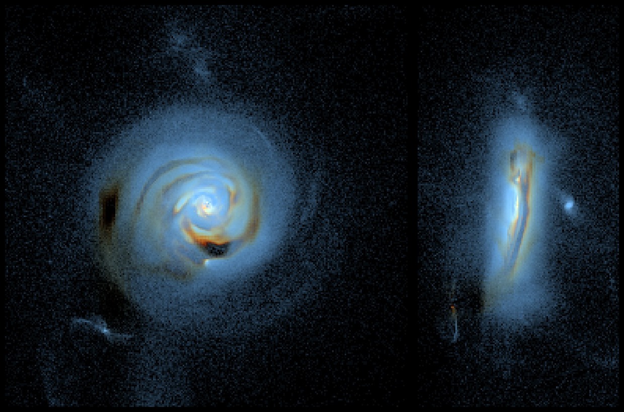
We included in Obelisk a subgrid model for the evolution of dust treated as a separate constituent to that of metals locked in the gas phase. The details of the model will be described in a future work (Dubois et al., in prep), and we present here the main features. Our model assumes that dust grains are released in the ISM via SN explosions, grow in mass via accretion of gas-phase metals, and are destroyed by SN explosions and via thermal sputtering. The figure below shows the resulting dust attenuation on a mock (rest-frame) image of a $z\sim 6$ galaxy with mass $M_\star = 4\times 10^{10}\,M_\odot$.

Specifically, we consider that all dust grains belong to one single population and are perfectly coupled to the gas (no dust drift relative to gas), so that they can be described with only one scalar $D$ describing the local dust mass fraction (this is similar to the approach taken by e.g. McKinnon et al. (2017) and Li et al. (2019)). This scalar is passively advected just as the metallicity $Z$, now representing the total metal mass fraction (in the gas phase as well as locked in the dust). We further neglect the size distribution of grains and assume that all grains have a unique size $a_{\mbox{d}}$. While the size distribution could in principle be followed in the model (e.g. McKinnon et al. 2018), this would come at a substantial memory overhead. In practice, we assumed that the grains have an average size of $a_{\mbox{g}} = 0.1\,\mu\mbox{m}$ and density $\mu_{\mbox{g}} = 2.4\,\mbox{g}\,\mbox{cm}^{-3}$. Finally, we stress that the dust is purely passive in our simulation: While in reality, a fraction $D/Z$ of the metals is locked into dust, we do not account for this when estimating the contribution of metal cooling.

When supernovae release metals in the ISM, we assumed that a fraction $f_{\mbox{d,SN}} = 50\%$ of these metals are in the form of dust and that the rest is in the gas phase. Because this parameter is very poorly constrained, we chose a value that falls in the middle of the range explored by Popping et al. (2017), who found that the value of $f_{\mbox{d,SN}}$ mostly affects the dust content of low-mass, low-metallicity galaxies. The high-velocity shocks produced by the SN explosion will also partially destroy the dust already present near the SN site. The mass $\Delta M_{\mbox{dest,SN}}$ of the dust destroyed in these events is related to the mass $M_{\mbox{s,100}}$ of gas shocked at above $100\,\mbox{km}\,\mbox{s}^{-1}$ via

$$\label{eq:dMdustSN} \Delta M_{\mbox{dest,SN}} = 0.3 \frac{M_{\mbox{s,100}}}{M_{\mbox{gas}}} M_{\mbox{d}},$$

where $M_{\mbox{gas}}$ is the local gas mass and $M_{\mbox{d}}$ is the local dust mass; meaning that 30% of the gas mass in the shocked gas is destroyed. We estimated the shocked gas mass by taking the Sedov solution in a homogeneous medium following McKee (1989):

$$\label{eq:Ms100} M_{\mbox{s,100}} \simeq \frac{E_{\mbox{SN}}}{0.736\ \left(100\,\mbox{km}\,\mbox{s}^{-1}\right)^2} \simeq 6800\, E_{\mbox{SN,51}}\,M_\odot.$$

We modelled the dust destruction via thermal sputtering following Draine & Salpeter (1979), with a destruction timescale given by (Draine 2011, chapter 25):

$$\label{eq:tsputtering} t_{\mbox{sput}} \simeq 0.1 \left(\frac{a_{\mbox{g}}}{0.1\,\mu\mbox{m}}\right) \left(\frac{n_{\mbox{gas}}}{\mbox{H}\,\mbox{cm}^{-3}}\right)^{-1} \left(1 + \left(\frac{T}{10^6\,\mbox{K}}\right)^{-3}\right)\,\mbox{Myr}.$$

In parallel, the dust content can grow in mass via accretion of metals from the gas phase. We estimate the competition between dust growth and destruction using an approach similar to that of (Dwek 1998, albeit simplified) or Novak et al. (2012):

$$\label{eq:dustmassgrowth} \dot{M}_{\mbox{growth}} = \left(1 - \frac{M_{\mbox{d}}}{M_{Z}}\right) \frac{M_{\mbox{d}}}{t_{\mbox{growth}}} - \frac{M_{\mbox{d}}}{t_{\mbox{sput}}},$$

where $M_Z$ the local metal mass in both the dust and gas phases, and $t_{\mbox{growth}}$ is the dust growth timescale

$$\label{eq:tgrowth} t_{\mbox{growth}} = 100 \frac{1}{\alpha(T)} \left(\frac{a_{\mbox{g}}}{0.1\,\mu\mbox{m}}\right)^{-2} \left(\frac{n_{\mbox{gas}}}{\mbox{H}\,\mbox{cm}^{-3}}\right)^{-1} \left( \frac{T}{20\,\mbox{K}} \right)^{-\frac{1}{2}} \,\mbox{Myr},$$

where $\alpha(T)$ is a the sticking coefficient of metals in the gas phase onto dust. The details of the impact of the choice of the sticking coefficient $\alpha$ are discussed in Dubois et al. (2021). Here, we used the results from laboratory experiments by Chaabouni et al. (2012):

$$\label{eq:stickingcoeff} \alpha(T) = 0.95\frac{1 + \beta\frac{T}{T_0}}{\left(1 + \frac{T}{T_0}\right)^\beta},$$

with $T_0 = 56\,\mbox{K}$ and $\beta = 2.22$. Overall, at temperatures below $T \simeq 3\times 10^4\,\mbox{K}$, dust growth happens faster than destruction via thermal sputtering.

We note here that the dust model is not coupled to the RHD on-the-fly but rather used for post-processing, for instance to assess the UV extinction: Going further would require a significantly more involved dust model (see e.g. Glatzle et al. 2019). To get an estimate of the impact of the UV extinction due to dust, we cast 192 rays from the centre of each galaxy and integrated the dust column density out to the virial radius of the host halo. We then converted this column density to an optical depth using the dust extinction law fits from Gnedin et al. (2008) for the Large Magellanic Cloud. This parametrization assumes that the dust extinction is proportional to the neutral hydrogen column density (their Eq.~5): We rescaled the neutral column density by the dust-to-gas ratio measured in our simulation along each line of sight to measure the dust optical depth.

References